4.2. Snowflake Algorithm

This section introduces the Snowflake algorithm, and gives an overview of how it works, as well as a description of it’s functionality and which parts of this I contributed to.

4.2.1. Approach

Snowflake belongs to a small number of phenotype prediction methods that aim to predict across many phenotypes and many genotypes. Although it’s designed primarily as a phenotype prediction algorithm, it also implicitly makes protein function predictions.

Snowflake aims to not only create phenotype predictions, but to create explanatory predictions, where the relevant parts of the molecular biology (missense variants falling in protein domains) can be traced back and used to explore the prediction further. In this sense it contrasts to the black-box approaches that are currently most successful.

The Snowflake phenotype prediction method works by identifying individuals who have unusual combinations of deleterious missense SNPs associated with a phenotype. The phenotype predictor uses only data about missense SNPs in coding regions of globular proteins, so it can only be expected to work well where phenotypes are determined primarily by these kinds of mutations.

This method combines conservation and variant effect scores using FATHMM[118], inference about function of protein domains using dcGO[114], and human genetic variation data from the 2500 genomes project[175] to predict phenotypes of individuals based on their combinations of missense SNPs.

4.2.2. How does it work?

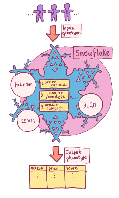
Fig. 4.2 Flowchart showing an overview of the phenotype predictor. Scores are generated per allele using SUPERFAMILY, VEP, FATHMM and dcGO for both the input genotype(s), and the background genotypes. These data points are then combined into a matrix, which is then clustered.

Fig. 4.2 shows how an overview of how Snowflake operates. One or more genotypes (in VCF or 23andMe format) are needed: this is the input cohort. The algorithm can then be divided into three main steps:

1. Score variants for deleteriousness, using FATHMM and VEP

2. Map variants to phenotype, using dcGO and SUPERFAMILY

3. Cluster individuals per phenotype and extract score, using IDOS. Each genotype will be compared against all others, including (optionally) a diverse background set from the 2500 Genomes Project[175].

Further detail on these steps is provided below.

4.2.2.1. SNPs are mapped to phenotype terms using DcGO and dbSNP

DcGO[114] is used to map combinations of protein domains to their associated phenotype terms, using a false discovery rate cut-off of \(10^{-3}\) or less. SNPs are therefore mapped to phenotype terms by whether they fall in a gene whose protein contains domains or combinations of domains that are statistically associated with a phenotype. In order to do this, DcGO makes use of SUPERFAMILY[113] domain assignments, and a variety of ontology annotations (GO[101], MPO[176], HP[177], DOID[178] and others).

Using DcGO means that phenotypes are only mapped to protein if the link is statistically significant due to the protein’s contingent domains. This leaves out some known protein-phenotype links, where the function may be due to disorder for example rather than protein domain structure.

Known phenotype-associated variants are therefore added back in using dbSNP[61].

4.2.2.2. SNPs are given deleteriousness scores using FATHMM

The phenotype predictor uses the unweighted FATHMM scores[118] to get scores per SNP for the likelihood of it causing a deleterious mutation. This is based on conservation of protein domains across all life, according to data from SUPERFAMILY[113] and Pfam[179].

This method gives SNPs the same base FATHMM score for being deleterious, no matter which phenotype we are predicting them for. It is therefore the combination of SNPs per phenotype, and their rarity in the population that determines the phenotype prediction score.

4.2.2.3. Comparison to a background via clustering

Individuals are compared to all others through clustering. This usually includes comparing each individual to the genetically diverse background of the 2500 genomes project[175].

Clustering is the task of grouping objects into a number of groups (clusters) so that items in the same cluster are similar to each other by some measure. There are many clustering algorithms, but most are unsupervised learning algorithms which iterate while looking to minimise dissimilarity in the same cluster. A number of options were implemented for the predictor, but for the time being at least, OPTICS is used as a default.

4.2.2.4. Phenotype score

The OPTICS clustering assigns each individual to a cluster (or labels them as an outlier). Depending on the phenotype term, the cluster is expected to either correspond to a haplogroup or a phenotype. In cases where the cluster refers to a haplogroup, we are interested in the outliers of all clusters, i.e. the local outlier-ness. In cases where the cluster is the phenotype, we are interested in the outlying cluster, i.e. the global outlier-ness.

A local score, \(L_{ij}\) can be defined as the average Euclidean distance from an individual to the centre of it’s cluster, or for individuals that are identified as outliers by OPTICS, 2 multiplied by the distance to the centre of the nearest cluster.

A global score \(G_{ij}\) can be defined as the distance of the cluster to the rest of the cohort.

TF-IDF

Term Frequency, Inverse Document Frequency is a common and basic measure in NLP which attempts to measure how representative a term (word) is of a document. It is defined by \(tfidf=tf(t,d) \cdot idf(t,D) = (f_{t,d}) \cdot (\frac{N}{abs{d \in D : t \in d}}) \) where \(f_{t,d}\) is the frequency of a term \(t\) in a document \(d\), \(N\) is the number of documents, and \({abs{d \in D : t \in d}\) is the number of documents containing the term.

The global-local score is designed to balance these sources of interest. It sums the two scores, adjusting the weighting by a cluster size correction factor, \(\mu_{\gamma}\): \(score_{ij}=L_{ij}+\mu_{\gamma} \cdot G_{ij}\)

Such that: \(\mu_{\gamma}=\frac{exp(\gamma \frac{n-n_j}{n})-1}{exp(\gamma)-1}\) where \(\gamma\) is a parameter representing how strongly we wish to penalise large clusters, \(n\) is the over all number of individuals and \(n_j\) is the number of individuals in a cluster.

The global-local score was inspired by the tf-idf score popular in Natural Language Processing bag-of-word models.

4.2.3. Functionality

Snowflake is implemented as a CLI tool, written in Python with the following commands:

• snowflake create-background

• snowflake create-consequence

• snowflake preprocessing

• snowflake predict

The functionality described above all happens within snowflake predict, but in order to use snowflake predict, there are also three commands which create files needed to run the predictor.

4.2.4. Features added to the predictor

As mentioned, the phenotype predictor was already prototyped when I began working on it. However, considerable time was spent developing, bug-fixing, and extending this prototype. Here, I describe my contributions to this in detail.

4.2.4.1. Different running modes

The original version of the phenotype predictor could only be ran one individual compared to a background set at a time. In order to allow for a wider range of inputs (which will be necessary to validate the predictor), support for a wider range of genotype formats and running modes was developed, including:

• Can be run with one person against a background

• Can be run with multiple people (VCF) against the background

• Can be run with or without the background set if there are enough people in the input set.

• Support for different 23andMe genotype file formats (from different chips).

As the predictor was developed to perform in different running modes, it became clear that it would be necessary to streamline the algorithm. This included parallelisation (possible due to the independence of different phenotype terms), and various data storage and algorithm adjustments.

Implementing these running modes and increases in efficiency was a collaborative effort between myself, Jan, and Ben.

4.2.4.2. Adding SNP-phenotype associations from dbSNP

As mentioned in the overview, using DcGO as the only SNP-phenotype mapping leaves out some known associations that are not due to protein domain structure. Adding dbSNP[61] associations to the predictor was one of my contributions to this software.

4.2.4.3. Dealing with missing calls

Genotyping SNP arrays often contain missing calls, where the call can not be accurately determined. This is an obstacle to the phenotype predictor if left unchecked as it can appear that an individual has a very unusual call when it is really just unknown. Since most people have a call, the missing call is unusual, and this is flagged.

The most sensible solution to this problem is to assign the most common call for the individual’s cluster (i.e. combination of SNPs). This prevents a new cluster being formed or an individual appearing to be more unusual than they are. However, there is a downside to this approach when there are many missing calls. Adding all missing calls to a cluster that was only slightly more common than the alternatives can lead to the new cluster containing the missing data dwarfing the others. To fix this, SNPs with many missing calls were discarded.

Alternatives such as assigning the most common call for that SNP only, or assigning an average score for that SNP dimension by carrying out a “normalised cut”[180] are untenable since they can create the same problem we are trying to overcome: the appearance of an individual having an unusual combination of calls.

4.2.4.4. Reducing dimensionality

Some phenotypes have large numbers of SNPs associated with them - too many to assign individuals to clusters. I added a dimensionality reduction step in the clustering, and tested different clustering methods designed for use on high-dimensional data. These changes are explained later in this Chapter.

4.2.4.5. Confidence score per phenotype

The phenotype predictor outputs a score for each person for each phenotype. Our confidence in these scores depends on the distribution of scores, as well as the scale of them. A distribution of scores with distinct groups of individuals is generally preferable, since most phenotypes that we are interested in are categorical or it is at least more useful to highlight phenotypes that can be predicted this way (i.e. if there are 100 groups with varying risk of a disease, that would be less useful than knowing there are 2 groups with high/low risk).

Fig. 4.3 An illustration of how the confidence score per phenotype is calculated.

I developed a simple method of prioritising predictions according to these requirements. A confidence score is achieved by plotting the ranked raw score and measuring the area between a straight line resting on this the most extreme points and the line itself, as illustrated in Fig. 4.3. Since this measure takes into account the size of the raw scores, these confidence scores can be compared across phenotypes.

Fig. 4.4 Ranked scores for DOID:1324 - the disease ontology term Lung Cancer (left) and HP:0008518 - the human phenotype ontology term for Absent/underdeveloped sacral bone (right). These represent an interesting and uninteresting distribution of scores, respectively.

Fig. 4.4 shows an example of an interesting and uninteresting distribution. These distributions mostly depend on the number, population frequency, and FATHMM score of the SNPs associated with the phenotype term.