4.5. Considerations for Clustering SNPs

In this section, I discuss the implementation of clustering and outlier detection methodologies for SNPs.

Snowflake is essentially a method for finding unusual combinations of SNPs, within sets of SNPs associated with a phenotype. Since there will be many rare combinations of SNPs just through randomness, the deleteriousness score (via FATHMM) decides which rare combinations are of interest.

The clustering takes place per phenotype, with the distinct phenotypes and the SNPs associated with them are chosen according to dcGO. This therefore determines how many dimensions (SNPs) we are clustering on for any given phenotype

4.5.1. Combinations of SNPs

Given \(N\) SNPs of interest, there are \(3^N\) different options for individual’s combinations of calls for biallelic SNPS, since there are three different options for each SNP WW wild-wild homozygous, MW/WM heterozygous, or MM mutant-mutant heterozygous.

For our purposes, heterozygous SNPs are considered the same whether they are mutant-wild MW or wild-mutant WM, since we assume they would create the same balance of proteins in a cell.

Linkage Disequilibrium

Linkage disequilibrium is the measure of how much more often alleles are found together than would be expected if they were randomly distributed. SNPs are not independent, and we wouldn’t expect alleles to be randomly distributed for many reasons, for example because:

• SNPs are inherited together through genetic linkage, due to being on the same gene or nearby genes from one another.

• we would expect combinations of SNPs to reflect the structure of the population, e.g. individuals who are geographically close to one another are more likely to have similar genetics.

• particular combinations of SNPs may be fatal or otherwise prevent people from passing them on.

The combinations of SNPs are not distributed randomly based only on the frequency of each SNP independently, this is what’s known in population genetics as linkage disequilibrium.

4.5.2. Choice of clustering methodology

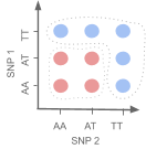
Fig. 4.7 A drawing indicating how the combinations of SNPs we might expect to cause disease would represent a non spherical relationship between SNPs.

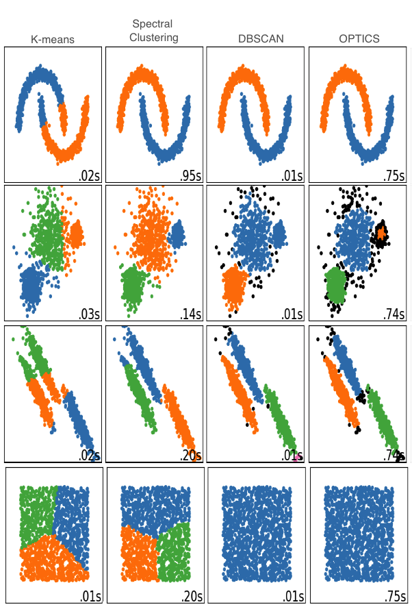
Fig. 4.8 Comparison illustrating differences between the implemented clustering methods. Image adapted from sklearn documentation[189].

The original implementation of the phenotype predictor used k-means clustering[190]. This wasn’t suitable for the predictor, since we expect combinations of SNPs to form non-spherical shapes (see Fig. 4.7), and k-means cannot achieve this (see Fig. 4.8).

Spectral clustering, DBSCAN (Density-Based Spatial Clustering of Applications with Noise), IDOS, OPTICS and LOF (Local Outlier Factor) were also implemented. This involved automation of parameter selection, to enable clustering to be performed automatically on thousands of phenotype terms. These methods have theoretical pros and cons with respect to the predictor. For example, OPTICS and DBSCAN do not need the number of clusters as an input, but instead require the minimum number of points required to form a cluster and a radius from each point to consider as part of a cluster, which has more meaning in this context. They also automatically output outliers to clusters, which will affect the resulting phenotype score, potentially in unseen ways - particularly as it is difficult to visualise high-dimensional data. OPTICS is the default setting, as in addition to not requiring a number of clusters, it can identify clusters of differing densities (a quality that DBSCAN lacks - as can be seen in the second row of Fig. 4.8). A final informed choice between these options requires a large benchmarking set.

4.5.2.1. Choice of distance metric

The phenotype predictor’s original distance metric was non-linear, such that the homozygous calls were further from each other than the distance via the heterozygous call, as shown in Fig. 4.9. Non-linear distance metrics mean that it is not possible to create a location matrix rather than a distance matrix. This is required for some types of clustering.

A linear distance metric which also captured the increased likelihood of homozygous alleles to be disease-causing (Fig. 4.10) was developed to enable this, and to better represent the biology. In this version, the popularity of an allele decides which homozygous call the heterozygous call is more functionally similar to.

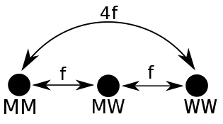
Fig. 4.9 Original non-linear distance metric. \(MM\) denotes homozygous mutant alleles, \(WW\) denotes homozygous wild type alleles, and \(MW\) denotes heterozygous alleles. The FATHMM score for the SNP \(f\), defines the distance between the wild type and mutant alleles.

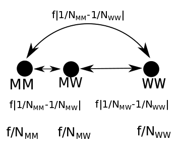
Fig. 4.10 Linear distance metrics. \(MM\) denotes homozygous mutant alleles, \(WW\) denotes homozygous wild type alleles, and \(MW\) denotes heterozygous alleles, and \(N\) represents the number of people with that allele call. The FATHMM score for the SNP \(f\), defines the distance between the wild type and mutant alleles.