8.4. Results and discussion

By harmonising the metadata of the four gene expression experiments, I have made it possible to query these four large data sets together, and I show an example of this. I have made the harmonised metadata for these experiments available for download through the Open Science Framework, here.

The combined data set represents 122 healthy tissues (all of which map to Uberon terms), over almost 20,000 samples, all which have consistent labelled sample information (age, development stage, sex). This wider variety of information can be used to increase coverage when gene expression data is needed for input to algorithms, which is done in the Filip chapter.

8.4.1. Example: Tissue-specific expression comparison

To illustrate the benefit of combining datasets, I will demonstrate that even the largest and most comprehensive gene expression experiments do not show all genes that are capable of expression being expressed.

from sklearn.metrics import cohen_kappa_score
import pandas as pd
import numpy as np
from myst_nb import glue

chosen_tissue_group = 'brain'  # the only tissue group in all experiments

design_file = 'data/design.csv'
design = pd.read_csv(design_file, sep=',', index_col=0)

tissue_names = pd.read_csv('data/tissue_groups_overlap.csv', index_col=0)
chosen_tissue_map = tissue_names[tissue_names['Group name'] == chosen_tissue_group]

# Print tissues within tissue group
chosen_tissues = chosen_tissue_map.index
design = design[design['Tissue (UBERON)'].isin(chosen_tissues)]
design['Tissue name'] = design['Tissue (UBERON)'].map(chosen_tissue_map['Tissue name'])
glue('num-brain-subtissues', len(design['Tissue name'].value_counts()))
brain_tissues = pd.DataFrame(design['Tissue name'].value_counts()).head()
brain_tissues.columns = ['Frequency in samples']
glue('brain-tissues-view', brain_tissues)

# Display breakdown by Experiment
breakdown_by_experiment = design.groupby('Experiment').count()[['Tissue name']]
breakdown_by_experiment.columns = ['Brain tissues']
glue('brain-design-view', breakdown_by_experiment)

I looked at the tissue group brain, since all experiments have tissues in this group (see Fig. 8.6). These samples represent 38 different brain tissues, Fig. 8.5 shows the most prevalent subtissue types.

	Frequency in samples
cerebral cortex	383
cerebellum	314
caudate nucleus	267
pituitary gland	249
nucleus accumbens	244

Fig. 8.5 The five most common subtissues making up the brain tissue group.

	Brain tissues
Experiment
FANTOM5	98
GTEx	2840
HDBR	480
HPA	3

Fig. 8.6 The breakdown of samples per source experiment in the brain tissue group.

To illustrate the fact that the different sources do not agree on whether or not genes are expressed, I first chose a random subset of 1000 genes from the combined dataset, then normalised the counts into TPM (using average transcript length from BioMart[264]). I then identified a TPM cutoff per experiment to reduce noise by graphing pairs of cerebral cortex samples in each experiment, looking for a threshold where like samples are not as similar as we would imagine.

# Read in expression data
combined_expression = pd.read_csv('data/combined/combined_subset.csv', index_col=0).astype(int)
combined_expression

# convert to TPM
def tpm(counts, lengths):
    rpk = counts.divide(lengths, axis='rows')
    scaling_factor = rpk.sum()
    tpm = (10**6)*rpk/scaling_factor
    return tpm.round(2)

lengths = pd.read_csv('data/mart_export_gene_lenths.txt')
lengths = np.ceil(lengths.groupby(['Gene stable ID']).mean()).astype(int)
lengths.columns = ['mean lengths']
combined_tpm = tpm(combined_expression, lengths['mean lengths'])

import plotly.graph_objects as go
from plotly.subplots import make_subplots

matched_samples = {}
for experiment in design['Experiment'].unique():    
    temp = design[design['Tissue name'] == 'cerebral cortex']
    matched_samples[experiment] = list(temp[temp['Experiment']==experiment].index)[:2]

log_combined_tpm = np.log2(combined_tpm + 1)

fig = make_subplots(
    rows=2, cols=len(design['Experiment'].unique()), 
    subplot_titles=design['Experiment'].unique(),
#     shared_yaxes=True,
)

step = 1
max_= 1000
bins = np.arange(0,max_, step)
colours = ['skyblue', 'limegreen', 'rgb(208, 32, 144)', 'darkorange']
colours_alpha = ['rgba(135, 206, 235, 0.1)', 
                 'rgba(50, 205, 50, 0.1)', 
                 'rgba(208, 32, 144, 0.1)',
                 'rgba(255, 140, 0, 0.1)']

for i, experiment in enumerate(design['Experiment'].unique()):
    sample1, sample2 = matched_samples[experiment]
    
    logtpm1 = log_combined_tpm[sample1]
    logtpm2 = log_combined_tpm[sample2]
    fig.add_trace(
        go.Scatter(x=logtpm1, y=logtpm2, 
                   mode='markers', 
                   name=experiment,
                   line=dict(color=colours_alpha[i]),
                   xaxis="x",
                   yaxis="y",
                   legendgroup=experiment,
                   

                  ),
        row =1, col=i+1,
    )
    
    tpm1 = combined_tpm[sample1]
    hist_y, bin_edges =  np.histogram(tpm1, bins=bins)
    fig.add_trace(
        go.Scatter(x=bin_edges[:-1], y=hist_y.cumsum(), 
                   mode='lines', 
                   name='Sample 1',
                   line=dict(color=colours[i], dash='dash'),
                   xaxis="x2",
                   yaxis="y2",
                   legendgroup=experiment,

                  ),
        row =2, col=i+1,
    )
    
    tpm2 = combined_tpm[sample2]
    hist_y, bin_edges =  np.histogram(tpm2, bins=bins)

    fig.add_trace(
        go.Scatter(x=bin_edges[:-1], y=hist_y.cumsum(), 
                   mode='lines', 
                   name='Sample 2',
                   line=dict(color=colours[i], dash='dot'),
                   xaxis="x2",
                   yaxis="y2",
                   legendgroup=experiment,
                  ),
        row =2, col=i+1,
    )
    fig.update_xaxes(title_text="log<sub>2</sub>(TPM+1)<br>sample 1", row=1, col=i+1)
    fig.update_xaxes(title_text="TPM", row=2, col=i+1, type='log')
    fig.update_yaxes(row=2, col=i+1, type='log')


fig.update_yaxes(title_text="log<sub>2</sub>(TPM+1)<br>sample 2",  row=1, col=1)
fig.update_yaxes(title_text="Number genes<br>with < TPM", row=2, col=1)
fig.update_layout({'width':720, 'height':600})

fig.show()

Fig. 8.7 Scatter plot (above) and cumulative histograms (bottom) showing two similar cerebral cortex samples from each experiment.

Table 8.2 Table showing the cut-offs chosen for each experiment.

Experiment	TPM cut-off
HDBR	5
FANTOM5	50
HPA	10
GTEx	25

In Fig. 8.7, I am looking for thresholds above which the samples correlate more strongly, as well as nonlinear behaviour in the low TPMs in the bottom plots, as described here[265]. I chose thresholds as shown in Table 8.2.

I then define “unexpressed” genes as genes which on average across samples in an experiment have a lower mean than this noise threshold, and calculated the genes that were unexpressed in brain samples from each experiment. Calculating the inter-rater reliability using Cohen’s Kappa (which adjusts for the probability of randomly rating samples the same way) between experiments reveals that there is moderate agreement between samples when using the per-experiment cut-offs chosen (see Fig. 8.8).

cut_offs = {
    'HDBR': 5,
    'FANTOM5': 10,
    'HPA': 10,
    'GTEx': 50,
}

def calc_kappas(cut_offs, experiments, design_df, exp_df):
    if not isinstance(cut_offs, dict):
        cut_off_dict = {}
        for experiment in experiments:
            cut_off_dict[experiment] = cut_offs
    else:
        cut_off_dict = cut_offs
        
    ratings = {}
    for experiment in experiments:
        samples = design_df[design_df['Experiment'] == experiment].index
        exp = exp_df[samples]
        expressed = (exp.mean(axis=1) > cut_off_dict[experiment]).astype(int)
        ratings[experiment] = expressed

    kappas = pd.DataFrame(index=experiments, columns=experiments)
    for i, e1 in enumerate(experiments):
        for j, e2 in enumerate(experiments):
            if i<j: 
                continue
            score = cohen_kappa_score(ratings[e1], ratings[e2])
            kappas.loc[e1, e2] = score
    return kappas.fillna('')

ck_cutoff = calc_kappas(cut_offs, design['Experiment'].unique(), design, combined_expression)
glue('ck-cutoff-view', ck_cutoff)

	HDBR	FANTOM5	HPA	GTEx
HDBR	1.000000
FANTOM5	0.575297	1.0
HPA	0.730815	0.720104	1.0
GTEx	0.763625	0.701627	0.875393	1.0

Fig. 8.8 Inter-rater reliability (Cohen’s Kappa) for unexpressed genes. The score can vary between -1 and 1, with scores below 0 representing random variation and 1 representing perfect agreement.

Although the different experiments do have moderate agreement, there is also a lot to be gained by combining them. Fig. 8.9 shows the overlap between unexpressed genes for brain, found in each experiment.

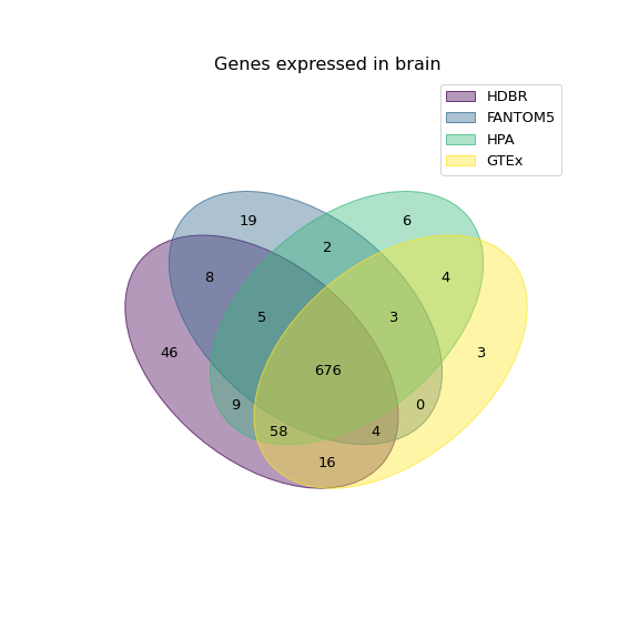
Fig. 8.9 Venn diagram showing the number of unique genes found in each experiment.

from venn import venn
from matplotlib import pyplot as plt

expressed = {}
for experiment in design['Experiment'].unique():
    samples = design[design['Experiment'] == experiment].index
    exp = combined_expression[samples]
    expressed[experiment] = set(exp[exp.mean(axis=1) > cut_offs[experiment]].index)

fig = venn(expressed)
plt.title('Genes expressed in brain', fontsize=16)
plt.savefig('../images/venn_brain.png')

plt.show()

8.4.2. Batch effects

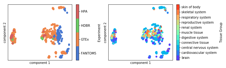
Fig. 8.10 PCA (Principal Components Analysis plot showing batch effects present in the combined dataset.

Batch effects are clearly present in the combined data set (see Fig. 8.10). I attempted batch effect correction using ComBat, however the PCA of the resulting data set did not cluster clearly by tissue type after batch effect removal which is a sign of “over correction”. ComBat requires a balanced experimental design which, as we have seen, is lacking in this combined dataset, so it is likely that is the reason for it’s unsuitability.

This means that the data set can not be used as-is for the purpose of measuring baseline expression (e.g. identifying housekeeping genes or measuring baseline tissue-specific gene expression). I explain some ideas for making the combined data set suitable for these types of analyses in future work.

However, by overcoming the data cleaning and standardisation necessary to have all datasets in the same format with the same sample metadata, the data can be used for analyses where batch and other sample metadata is used as covariates (e.g. differential expression of tissues). In its current iteration, it is also suitable for use in improving Filip, where the data set only needs to distinguish between presence and absence (as in the example above, this problem can be side-stepped by choosing a cut-off per experiment).

8.4.3. Combining omics data sets is an opportunity to improve existing resources

While a great deal of careful work has clearly been spent on making the datasets used in this analysis available and useful to researchers such as myself, there were still many barriers to their use in this circumstance. This ranged from mislabelled samples, to missing information, to having to seek data about the same experiment from multiple different sources (as we saw in Section 7.5). It is reassuring that the data issues that were discovered had clear pathways for reporting, and that some of them have already resulted in changes to the files used. In particular, I think it’s important that key information that we know affects gene expression such as age, developmental stage, and sex are made available with the data set and preferably in a standardised format across experiments.

8.4.4. Future Work

The main piece of future work that I anticipate doing is using the combined dataset to improve the coverage of the Filip prediction filter.

8.4.4.1. Mapping improvements

There are also some mapping improvements which might improve the quality of the data set as a resource for other people.

Multiple membership of tissues and cells It is sometimes appropriate for samples to map to two apparently distinct Uberon terms. For example, leukocytes are known to be part of the immune system, but are found in the blood. In the FANTOM mapping, they would be mapped by name to blood, but by ontology to immune system. In this case, we could imagine mapping to two Uberon terms rather than defaulting to where the cells were collected, since researchers interested in blood or the immune system would both like to access the information.

In addition, it would be preferable to map simultaneously to tissue and cell type, since this enables researchers to, for example, make queries about expression about the same cell types in different tissue locations, query the data set against scRNA-seq data, or simply find cell as well as tissue specific information. This could be achieved partly with relative ease by using the ontological mapping between CL and Uberon. Improvement of the CL-Uberon mapping would then allow for a complete understanding of which cell types are in a tissue, but not their relative abundances.

Cell type deconvolution: In order to understand the relative abundances of cell types in each sample, a cell type deconvolution programme (e.g. CIBERSORT[266], BSEQ-sc[267], or MuSiC[268]) could be used. These algorithms estimate percentages of cell types making up a tissue. This would require the input of a large scRNA-seq data set as input, and there doesn’t yet exist enough diversity to deconvolve all tissue types. As well as improving the mapping, this is likely to improve the quality and variety of batch effect correction methods available.

8.4.4.2. Batch effect removal

Many popular batch-effect removal techniques (e.g. ComBat and ComBat-Seq[269]) require a balanced experimental design, which this combined dataset does not have. It is not clear, however, to what extent this may affect their performance. Some alternative methods are not as sensitive to this requirement, e.g. Mutual Nearest Neighbour (MNN)[270], which was developed for scRNA-seq data. No batch-effect removal method is designed specifically for this kind of scenario, so it would be sensible to do a simulation study to test their suitability; some preliminary work towards this goal can be found in the appendix.

8.4.4.3. Tissue-specific vs cell specific

As the number of scRNA-seq experiments increases, including them in a combined dataset of tissue-specific expression will become more statistically viable. A prerequisite of including scRNA-seq data would be the use of an alternative batch effect removal algorithm that is suitable for single cell data (e.g. MNN). It would be interesting to compare how the expression of cells which can exist in multiple tissue types differs across those different tissue types, and to investigate whether some gene expression is truly tissue-specific rather than cell-type specific.